Basic Simulation

In this tutorial, we will model the reaction A + 1/2 B₂ AB using simplified placeholder values for demonstration purposes.

Tip

For anyone starting to work with MKMCXX or with microkinetic simulations in general, this tutorial is an excellent starting point which covers the basic features and settings of MKMCXX, including plotting and data interpretation.

Input file

Current MKMCXX 3 input files use the newer MKX block syntax. A complete input file typically contains:

Optional let statements for reusable values
A components { ... } block describing the species in the system
A reactions { ... } block describing the elementary steps
A simulation { ... } block describing solver settings, analyses, and run conditions
An output { ... } block describing how results should be written

The complete input file used in this tutorial is also available as examples/basic/input.mkx in the source tree.

Below, we will address each of these sections.

Compounds

We assume the reaction proceeds as follows. Species A adsorbs molecularly on the catalytic surface, while B₂ adsorbs dissociatively. These adsorption steps produce the surface species A and B, respectively. The adsorbed species A and B can then combine to form AB, releasing an empty site. Finally, AB desorbs from the surface to regenerate the active site.

For this model, we therefore require three gas-phase species (A, B2, AB) and four surface species (A*, B*, AB*, and *, the latter representing an empty site).

Tip

We use the suffix * to indicate an adsorbed species. Later, when we will be plotting the results, we can use this suffix to identify adsorbed species using their labels.

For an optimal reaction, we assume that the gas phase pressures of A and B₂ are according to their stoichiometric ratio, i.e. 1 atm for A and 0.5 atm for B₂.

The components block thus looks as follows:

components {
  A   {phase=gas, init=1.0, role=reactant},
  B2  {phase=gas, init=0.5, role=reactant},
  AB  {phase=gas, init=0.0, role=product, tags=[key]},

  A*  {phase=surface, init=0.0},
  B*  {phase=surface, init=0.0},
  AB* {phase=surface, init=0.0},
  *   {phase=surface, init=1.0, tags=[emptysite]}
}

In this block, we indicate for each component:

Its label
Its starting concentration through the init=value field.
Its phase via phase=gas or phase=surface.
Its role in the gas phase via role=reactant or role=product.
Optional tags. For sensitivity analysis, at least one gas-phase product should be marked with tags=[key]. Here, we choose AB as the key compound.

Note

Always define at least one key compound, else any kind of sensitivity analysis will fail.
It is strongly recommended to set phase and, for gas-phase components, also set role.
Marking the empty site with tags=[emptysite] makes the intent of the model explicit and keeps the input easier to read.

Reactions

To model the reactions, we will introduce four elementary reaction steps, corresponding to adsorption/desorption of the reactants and products and a surface reaction where A and B are combined. As indicated above, A and AB will adsorb/desorb molecularly and B2 will adsorb/desorb dissociatively/recombinatorily. This yields the following reactions block:

let asite = 1e-20
let arr_base = {Vf=1e13, Vb=1e13}

reactions {
  {A}+{*}=>{A*} @ HertzKnudsenDefault(Asite=asite, m=12, theta=1.0, sigma=1, S=1, Edes=120e3) {tags=[drc]},
  {B2}+2{*}=>2{B*} @ HertzKnudsenDefault(Asite=asite, m=28, theta=1.0, sigma=1, S=1, Edes=80e3) {tags=[drc]},
  {AB}+{*}=>{AB*} @ HertzKnudsenDefault(Asite=asite, m=26, theta=1.0, sigma=1, S=1, Edes=50e3) {tags=[drc]},
  {A*}+{B*}=>{AB*}+{*} @ ArrheniusDefault(*arr_base, Eaf=120e3, Eab=80e3) {tags=[drc]}
}

In current MKMCXX syntax, each reaction entry consists of:

Species labels are enclosed in curly brackets {...}.
- Example: {A}, {B2}, {A*}, {*}
Stoichiometric factors are written in front of the label.
- Example: 2{B*} means two adsorbed B atoms.
The reaction arrow => separates reactants (left) from products (right). Note that all elementary reaction steps are assumed to be microscopically reversible, so the reactions will always be evaluated in both forward and backward direction. Thus, you only have to define them once.
The @ ModelName(...) suffix selects the kinetic model and passes its parameters.
Optional metadata can be appended as an object literal, for example {tags=[drc]}.

The let statements shown above are optional but useful. They allow you to reuse values such as site area (asite) and shared Arrhenius parameters (arr_base) without repeating them on every line.

In this example, we consider two types of elementary reaction models:

HertzKnudsenDefault:
Used for adsorption and desorption steps. This model applies the Hertz–Knudsen equation to calculate rates based on molecular flux, sticking probability, site area, and desorption energy. It is typically chosen for gas–surface interactions.
ArrheniusDefault:
Used for surface reactions between adsorbed species. This model follows the Arrhenius equation, defined by (temperature-independent) pre-exponential factors and activation energies for forward and backward reactions. It is typically chosen for bond-forming and bond-breaking steps on the surface.

Warning

Although elementary reaction steps are microscopically reversible, elementary reaction steps for which the HertzKnudsenDefault model is being used need to be written such that the gas-phase components are on the left-hand side of the reaction.

Hertz-Knudsen

For Hertz-Knudsen reaction, by default, the following forms for the reaction rate constants are assumed.

\[ k_{f} = \frac{pA_{\text{site}}}{\sqrt{2 \pi m k_{b} T}} S \]

and

\[ k_{b} = \frac{k_{b}T^{3}}{h^{3}} \frac{A_{\text{site}}(2 \pi m k_{b})}{\sigma \theta_{\text{rot}}} \exp \left( -\frac{\Delta E_{\text{des}}}{k_{b}T} \right) \]

Given these equations, the user needs to define, inside HertzKnudsenDefault(...), the following parameters:

Asite: Active site surface area in m^-2.
m: Mass of the species in amu. (atomic units)
theta: Rotational temperature in K
sigma: Symmetry factor (dimensionless)
S: Sticking coefficient (dimensionless)
Edes: Desorption energy in J/mol

Note

The desorption energy is the energy that needs to be invested to remove the species from the surface. As such, this should in principle be a positive value.

Arrhenius

For Arrhenius equations, we use the following form for the reaction rate constants. This functional form assumes that the pre-exponential factor is temperature-independent. This is an approximation.

\[ k_{f} = \nu_{f} \exp \left( -\frac{\Delta E_{\text{a,f}}}{RT} \right) \]

and

\[ k_{b} = \nu_{b} \exp \left( -\frac{\Delta E_{\text{b,f}}}{RT} \right) \]

Given these equations, the user needs to define, inside ArrheniusDefault(...), the following parameters:

Vf: Pre-exponential factor in the forward direction in s^-1.
Vb: Pre-exponential factor in the backward direction in s^-1
Eaf: Forward barrier in J/mol.
Eab: Backward barrier in J/mol.

Tip

A typical ballpark value for the forward and backward pre-exponential factors can be derived from the equation \(k_{b}T/h\) which is roughly 1e13 s^-1.

Simulation

In current v3 syntax, global simulation settings, analyses, and the list of run conditions live together in a simulation block. For a thermal transient simulation, the most important pieces are:

model: The physical simulation mode, here thermal.
solver: The numerical solver configuration.
analyses: Additional sensitivity analyses to compute.
conditions: The list of temperatures or other per-run overrides.

Each condition in the list must define at least:

T: The simulation temperature in K.

The solver typically defines the default numerical settings:

t_end: The integration time in s.
atol: Absolute tolerance for the ODE solver.
rtol: Relative tolerance for the ODE solver.
steady_state_threshold: Optional early-stop criterion. If the largest absolute derivative in the system, Max|dy/dt|, falls below this value, the transient run is considered sufficiently close to steady state and can stop before reaching t_end.

The simulation is performed by time-integrating the system of ordinary differential equations that represent the elementary reaction steps. Initial conditions are taken from the init=value fields in the components block. By default, the simulation begins with an empty catalytic surface as the initial state. Gas-phase species are held constant, corresponding to a finite-conversion simulation. Time integration is carried out using finite time steps. The solver adjusts the step size dynamically, guided by user-defined relative and absolute tolerances. These tolerances ensure that increasing the step size, improving efficiency, does not introduce errors larger than the specified thresholds.

We use the following setup to explore the system between T = 350 K and T = 1200 K using steps of 25 K. We use an absolute and relative tolerance of 1e-8 throughout, t_end = 1e8 s of simulation time, and steady_state_threshold = 1e-4. For the first two temperatures, we tighten the tolerances further to 1e-10. This illustrates a useful practical point: some individual conditions can be numerically more challenging than the rest of the sweep, and it is perfectly reasonable to set stricter tolerances only for those cases.

simulation {
  baseline @ transient_solve(
    model=thermal,
    solver={method=cvode_bdf, atol=1e-8, rtol=1e-8, t_end=1e8, steady_state_threshold=1e-4},
    analyses=[
      {type=reaction_orders, enabled=true},
      {type=drc, enabled=true},
      {type=eapp, enabled=true}
    ],
    conditions=[
      {T=350,  rtol=1e-10, atol=1e-10},
      {T=375,  rtol=1e-10, atol=1e-10},
      {T=400},  {T=425},  {T=450},  {T=475},  {T=500},  {T=525},
      {T=550},  {T=575},  {T=600},  {T=625},  {T=650},  {T=675},
      {T=700},  {T=725},  {T=750},  {T=775},  {T=800},  {T=825},
      {T=850},  {T=875},  {T=900},  {T=925},  {T=950},  {T=975},
      {T=1000}, {T=1025}, {T=1050}, {T=1075}, {T=1100}, {T=1125},
      {T=1150}, {T=1175},
      {T=1200}
    ]
  )
}

Tip

For the simulation time t_end, use a value significantly high by which you can reasonably assume that the system has reached its steady-state condition. Of course, always check it by looking into the time-profiles.
steady_state_threshold controls whether a transient run may stop early. Once Max|dy/dt| drops below this value, the run is reported as steady_state. If the threshold is not reached before t_end, the run stops at final_time instead. Smaller values impose a stricter steady-state criterion; larger values allow earlier termination.
Good default values for the absolute and relative tolerances are 1e-8. In practice, values far below ~1e-15 are rarely useful in a double-precision build because they are already at or beyond the meaningful floating-point resolution of the solver.
If one temperature or pressure point does not converge as smoothly as the rest, you do not need to change the whole sweep immediately. You can add rtol and atol directly to that specific entry in conditions, as shown above for T=350 K and T=375 K.
Why this helps: the transient solver controls its time-step based on the estimated local integration error. Near some operating points, the system may become effectively stiffer, exhibit sharper coverage changes, or pass through very small intermediate values. Tighter tolerances force the solver to take smaller, more careful steps there, which can improve robustness and produce cleaner steady-state estimates.

Output

The results of the simulation are written to a permanent medium (e.g. hard drive). In the output block, we indicate which storage formats should be used and which folder should receive the results. If multiple storage formats are specified, the simulation results are stored in all of them. In the example below, we write the results in all three supported formats and keep the default output folder name results.

output {
  formats=[excel, tabdelim, hdf5],
  folder="results"
}

The supported formats are as follows:

HDF5: A High-performance data management and storage suite that efficiently stores heterogeneous data in a single file.
EXCEL: MS-XLSX Office Open XML Spreadsheet Format. Can be opened in Microsoft Excel or other spreadsheet software supporting this format. The format is also supported by the Python Data Analysis Library (pandas).
TABDELIM: A simple flat-text style format using tabs as the delimiting character.

Running the simulation

By placing all of these sections inside a single .mkx file, we can start the simulation by executing the following one-liner from a terminal application.

<path to mkmcxx executable> -i <path to input file>

Note

If you have made changes to the input file and wish to rerun the simulation, overwriting previous results, you need to add the -f instruction on the command line.

Typical output of the program is similar to the excerpt shown below. This example was produced by running the bundled examples/basic/input.mkx case with the packaged executable.

$ <path-to-executable>/mkmcxx -i examples/basic/input.mkx -f
================================================================================

MKMCXX Version: 3.1.0
Compiled with: GNU 15.2.0
Build type: Release
Compiler flags: -fno-fast-math -ffp-contract=off -frounding-math
                -fexcess-precision=standard -fno-unsafe-math-optimizations
                -fno-associative-math -fno-finite-math-only -fno-reciprocal-math
                -O3 -DNDEBUG -flto=auto
Float type: double
Float size: 8 bytes
Float precision: 53 bits
Build time: 2026-04-10 14:08:30
Author: Ivo Filot <i.a.w.filot@tue.nl>

================================================================================
CPU Vendor: GenuineIntel
CPU Model: Intel(R) Core(TM) i9-10900K CPU @ 3.70GHz
Logical Threads: 20
Total RAM: 62.7336 GB
OS: Ubuntu 24.04.4 LTS
Kernel: 6.6.87.1-microsoft-standard-WSL2
================================================================================
Reading input from: ./examples/basic/input.mkx
Done reading input file.

=== Execution Plan ===
Components: 7
Reactions:  4
Simulations: 1
Outputs:    EXCEL, HDF5, TABDELIM
Output dir: results
 - baseline [model=transient_solve, runs=35, analyses=drc, eapp, reaction_orders]

Running simulation 'baseline'...
[Orchestrator] Launching 1155 jobs using 20 threads.
✓ Running: 0   ✓ Completed: 1155   ○ Queued: 0
[Orchestrator] All jobs completed successfully.


=============================================================================
                           COMPUTATION TIME REPORT                           
=============================================================================
Total jobs executed:              1155
Cumulative computation time:      1.4113 s
Average job time:                 0.0012 s
Min/Max job time:                 0.0001 / 0.0244 s

Type       Jobs   Total[s]     Avg[s]     Min[s]     Max[s]
-----------------------------------------------------------------------------
CORE         35     0.0855     0.0024     0.0003     0.0244  Threads: 19
ORDER       420     0.4853     0.0012     0.0001     0.0075  Threads: 20
DRC         560     0.6521     0.0012     0.0002     0.0072  Threads: 20
EACT        140     0.1884     0.0013     0.0002     0.0063  Threads: 20
-----------------------------------------------------------------------------


=============================================================================
                       COMPUTATION CONVERGENCE REPORT                        
=============================================================================
Job ID    SimID       End t         Stop          Threshold     Max|dy/dt|    
------------------------------------------------------------------------------
1         T=350       2.512e-01     steady_state  1.000e-04     8.391e-05     
2         T=375       1.000e-01     steady_state  1.000e-04     6.885e-05     
3         T=400       3.981e-02     steady_state  1.000e-04     7.217e-05     
4         T=425       1.585e-02     steady_state  1.000e-04     4.482e-05     
5         T=450       2.512e-03     steady_state  1.000e-04     3.945e-06     
6         T=475       7.943e-04     steady_state  1.000e-04     1.897e-05     
...
35        T=1200      1.000e+08     final_time    1.000e-04     1.283e-02     
------------------------------------------------------------------------------


=============================================================================
                          COMPUTATION ERROR REPORT                           
=============================================================================
No errors were encountered!
-----------------------------------------------------------------------------

Writing results in HDF5 format.
Writing results in TABDELIM format.
Writing results in EXCEL format.

================================================================================
All done!
Total simulation (wallclock) execution time: 1.651 seconds
Output [baseline]: /path/to/results
================================================================================

The program output contains:

Program and build (compilation) information
- Version number, compiler and flags, build type, floating-point precision, and build time.
System details
- CPU vendor and model, number of threads, total RAM, operating system, and kernel.
Input and execution summary
- Name of the input file, parsed execution plan, number of runs, enabled analyses, and output formats.
Execution log
- Notes on overwritten directories, job orchestration, number of jobs launched, queued, and completed.
Computation time report
- Total number of jobs executed
- Cumulative, average, minimum, and maximum job times
- Breakdown by job type (e.g. CORE, ORDER, DRC, EACT), including per-thread statistics
Convergence report
- For each temperature point, whether the run stopped because steady state was reached or because t_end was reached first.
- The reported Max|dy/dt| value is useful for judging how close the run is to steady state at the stop point.
- If Max|dy/dt| drops below steady_state_threshold, the run is labeled steady_state; otherwise it continues until t_end and is labeled final_time.
Error report
- A compact summary indicating whether any runs failed.
Output files
- Confirmation of results written in HDF5, tab-delimited, and Excel formats.
Completion summary
- Total wall-clock execution time and the location of the output folder.

Results, plotting and interpretation

The results of the simulation are written to a separate results folder located in the current working directory. To visualize and interpret the results, it is recommended to make use of small Python scripts. Here, we provide examples making use of the h5py library which can efficiently read out a hdf5 output file.

Concentrations

To visualize the surface concentration as function of temperature, we use the following small Python script

import h5py
import matplotlib.pyplot as plt

with h5py.File('results/results.h5', 'r') as f:
    if 'aggregated/kinetics/concentrations' in f:
        plt.figure(dpi=144)
        dset = f['aggregated']['kinetics']['concentrations']
        data = dset[:]
        for i in range(data.shape[1]-1):
            label = dset.attrs['column_labels'][i+1]
            if '*' in label:
                plt.plot(data[:, 0], data[:, i + 1], '-o', label=label)
        plt.grid(linestyle='--')
        plt.legend()
        plt.xlabel('Temperature [K]')
        plt.ylabel('Surface concentration [-]')

This script opens the .h5 file and looks for the data entry corresponding the concentrations as function of temprature (aggregated/kinetics/concentrations). If found, a graph is constructed where we loop over the compounds and visualize only those compounds which have a * in its label, i.e., only for the surface compounds. The reason we do not visualize the gas-phase compounds is because they are kept static throughout the simulation and are thus not relevant to investigate. The graph produced by this script is found below.

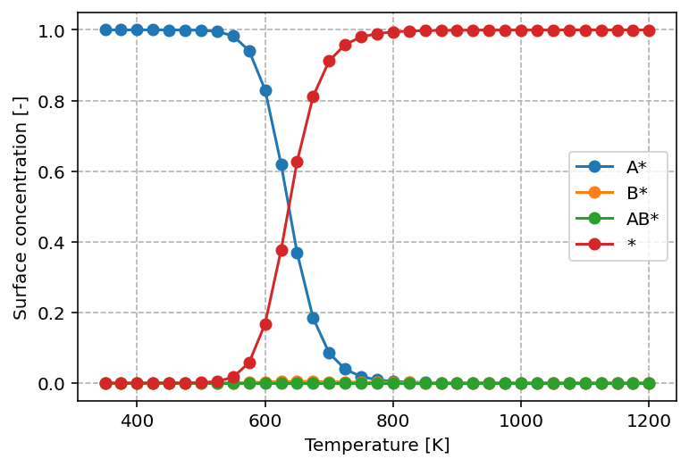
Concentrations as function of temperature

From this graph, we can readily see that at low temperature, the surface is predominantly covered by A*, in line with its higher desorption energy of 120 kJ/mol versus 80 kJ/mol for B*. With increasing temperature, we observe that the surface concentration of A* decreases in favor of *. This is a common pattern. With increasing temperature, desorption and reaction become more facile and the result is that AB* can be rapidly formed and desorbed from the surface by which the surface becomes gets increasingly more free sites.

Derivatives

One core observable is how temperature then affects the turn-over-frequecy for this catalyst. To investigate this, we need to look into the derivatives, which is another entry in the results.h5 file. To visualize it, we make use of the following Python script

import h5py
import matplotlib.pyplot as plt

with h5py.File('results/results.h5', 'r') as f:
    if 'aggregated/kinetics/derivatives' in f:
        plt.figure(dpi=144)
        dset = f['aggregated']['kinetics']['derivatives']
        data = dset[:]
        for i in range(data.shape[1]-1):
            label = dset.attrs['column_labels'][i+1]
            if '*' not in label:
                plt.plot(data[:, 0], data[:, i + 1], '-o', label=label)
        plt.grid(linestyle='--')
        plt.legend()
        plt.xlabel('Temperature [K]')
        plt.ylabel('TOF [-]')

The graph produced by the above script is shown below.

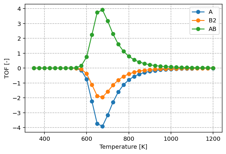
Derivatives as function of temperature

The graph shows that reactants are consumed and products are formed according to their stoichiometric ratios, with A : B₂ : AB = 1 : 1/2 : 1. The turnover frequencies (TOF) exhibit a maximum as a function of temperature, which is a typical result in heterogeneous catalysis and reflects the Sabatier principle. At low temperatures, the available thermal energy is insufficient to overcome reaction barriers. At high temperatures, adsorbates desorb rapidly instead of remaining on the surface to react. As a result, the highest TOF is achieved only at intermediate temperatures.

Note

Comparing this result to the concentrations profile, observe that this optimum in reactivity corresponds to the situation where A* and * are roughly in equal ratios.

Reaction orders

Both experimentally and through simulation, an important kinetic property that can be determined is the reaction order. The reaction order describes how the overall reaction rate responds to changes in the partial pressure of a gas-phase species. In other words, it measures the sensitivity of the forward rate to variations in the concentration of a particular reactant.

Mathematically, the reaction order with respect to species x is defined as

\[ n_{x} = p_{x} \, \frac{\partial \ln r^{+}}{\partial p_{x}} \]

where

\(p_{x}\) is the partial pressure of species x
\(r^{+}\) is the forward reaction rate

A positive reaction order indicates that increasing the pressure of species x accelerates the reaction, while a negative value indicates an inhibitory effect. Reaction orders are often non-integer values in heterogeneous catalysis, reflecting the complex interplay between adsorption, surface reactions, and desorption.

import h5py
import matplotlib.pyplot as plt

with h5py.File('results/results.h5', 'r') as f:
    if 'aggregated/kinetics/derivatives' in f:
        plt.figure(dpi=144)
        dset = f['aggregated']['sensitivity']['orders']
        data = dset[:]
        for i in range(data.shape[1]-1):
            label = dset.attrs['column_labels'][i+1]
            if '*' not in label:
                plt.plot(data[:, 0], data[:, i + 1], '-o', label=label)
        plt.grid(linestyle='--')
        plt.legend()
        plt.xlabel('Temperature [K]')
        plt.ylabel('Reaction order [-]')

The graph produced by the script above looks as follows

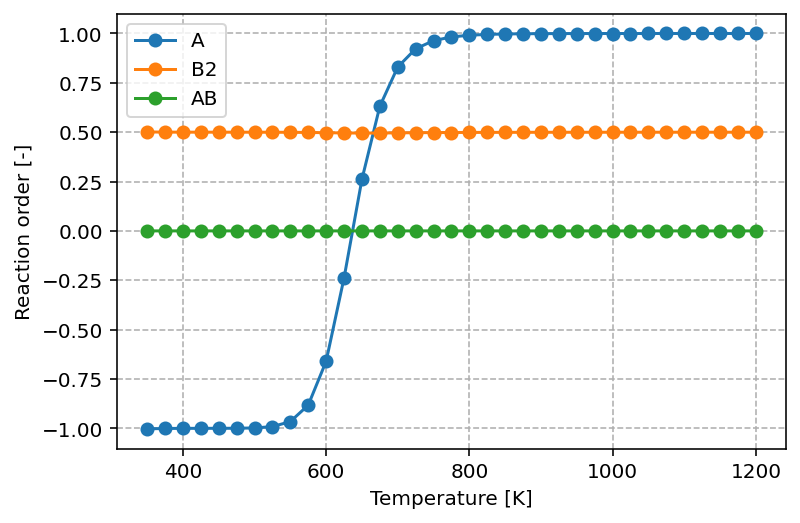
Reaction order as function of temperature

The graph shows that at low temperatures the reaction order with respect to A is negative (–1). This means that increasing the partial pressure of A actually inhibits the overall reaction rate, which can be understood as a consequence of surface poisoning: excess adsorption of A blocks active sites that would otherwise participate in the formation of products. As the temperature increases, the reaction order in A rises and eventually reaches +1. In this regime, higher partial pressures of A promote the reaction, consistent with A becoming the rate-controlling reactant.

For B₂, the reaction order remains constant at 0.5 across the entire temperature range. This fractional order suggests that the rate depends on the square root of the B₂ pressure, which is typical for dissociative adsorption processes where two surface sites are required. For AB, the reaction order is 0.0, indicating that the rate is independent of the partial pressure of AB. This behavior is expected for a product, as its presence in the gas phase does not directly influence the forward rate of reaction.

Apparent activation energy

Another key kinetic property that can be obtained from both experiment and simulation is the apparent activation energy. The apparent activation energy characterizes how the overall reaction rate changes with temperature. Unlike the intrinsic activation energy of an individual elementary step, the apparent activation energy reflects the combined influence of all relevant processes, including adsorption, surface reactions, and desorption. As such, it provides valuable insight into which steps are rate-controlling under given operating conditions.

Mathematically, the apparent activation energy is defined as

\[ E_\text{app} = RT \, \frac{\partial \ln r^{+}}{\partial T} \]

where

\(R\) is the universal gas constant
\(T\) is the temperature
\(r^{+}\) is the forward reaction rate

A higher apparent activation energy indicates stronger temperature dependence of the reaction rate, while a lower value suggests that other effects, such as adsorption equilibria, are compensating for the intrinsic barrier. In heterogeneous catalysis, the apparent activation energy can therefore differ significantly from the activation energy of the elementary surface reaction, and its variation with conditions often reveals mechanistic details about the catalytic cycle.

Via the Python script as shown below, we can visualize the apparent activation energy

import h5py
import matplotlib.pyplot as plt

with h5py.File('results/results.h5', 'r') as f:
    if 'aggregated/kinetics/derivatives' in f:
        plt.figure(dpi=144)
        dset = f['aggregated']['sensitivity']['eapp']
        data = dset[:]
        for i in range(data.shape[1]-1):
            label = dset.attrs['column_labels'][i+1]
            plt.plot(data[:, 0], data[:, i + 1] / 1000, '-o')
        plt.grid(linestyle='--')
        plt.xlabel('Temperature [K]')
        plt.ylabel('Apparent activation energy [kJ/mol]')

which yields the following graph

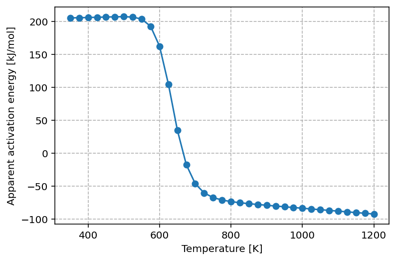
Apparent activation energy as function of temperature

The graph shows that at low temperature the apparent activation energy is approximately 200 kJ/mol. This value can be rationalized by considering the elementary steps required for the reaction to proceed under these conditions. Since the surface is almost fully covered by A, one A must first be removed, which requires about 120 kJ/mol. The subsequent adsorption of half a B₂ molecule stabilizes the system, releasing roughly 40 kJ/mol. Together with the intrinsic reaction barrier of 120 kJ/mol, this leads to an effective apparent activation energy close to 200 kJ/mol.

As the temperature increases, the surface becomes less saturated with A*, and more vacant sites are available. This lowers the apparent activation energy, reflecting a kinetically more favorable regime where surface crowding is no longer the primary limitation.

At the optimal reaction temperature, the apparent activation energy approaches zero. This corresponds to the maximum in the turnover frequency (TOF), where the rate is locally insensitive to changes in temperature—analogous to probing the extremum of a function.

At even higher temperatures, the apparent activation energy becomes negative. In this regime, increasing the temperature reduces the overall reaction rate because adsorbates desorb too rapidly to participate effectively in surface reactions. Consequently, lowering the temperature actually enhances the rate. This inversion is a hallmark of the Sabatier principle, which predicts that maximum catalytic activity occurs only within an intermediate temperature (or binding energy) window.

Degree of rate control

Another valuable kinetic descriptor is the Degree of Rate Control (DRC).
The DRC quantifies how sensitive the overall reaction rate is to changes in the rate constant of an individual elementary step. In other words, it measures how much "control" each step exerts over the overall kinetics of the catalytic cycle.

Mathematically, the DRC of step i is defined as

\[ \chi_i = \frac{k_i}{r} \, \frac{\partial r}{\partial k_i} = \frac{\partial \ln r}{\partial \ln k_{i}} \]

where

\(k_i\) is the rate constant (both forward and backward) of elementary step i
\(r\) is the overall reaction rate

The DRC takes values between 0 and 1 in many practical cases. A value close to 1 indicates that the step is strongly rate-controlling: small changes in its rate constant directly scale the overall rate. A value close to 0 means the step has little influence on the kinetics under the given conditions. Interestingly, negative values can also occur, implying that accelerating that step would actually reduce the overall reaction rate (e.g. by shifting equilibria or surface coverages unfavorably).

The DRC thus provides a powerful tool for mechanistic analysis: it identifies which elementary steps are kinetically relevant, guides catalyst design by pointing to critical barriers, and helps explain why apparent kinetic parameters vary with conditions.

The following Python script extracts the DRC results from results.h5 and visualizes it.

import h5py
import matplotlib.pyplot as plt

with h5py.File('results/results.h5', 'r') as f:
    if 'aggregated/kinetics/derivatives' in f:
        plt.figure(dpi=144)
        dset = f['aggregated']['sensitivity']['drc']
        data = dset[:]
        for i in range(data.shape[1]-1):
            label = dset.attrs['column_labels'][i+1]
            plt.plot(data[:, 0], data[:, i + 1], '-o', label=label)
        plt.grid(linestyle='--')
        plt.legend()
        plt.xlabel('Temperature [K]')
        plt.ylabel('Degree of rate control [-]')

DRC as function of temperature

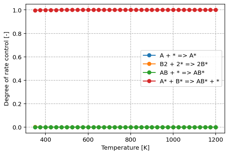
From the graph above, we can see that only one elementary step—the surface reaction—has a significant impact on the overall kinetics. Its DRC value is equal to 1, which means that this step fully controls the reaction rate under the given conditions. In practical terms, any change to the rate constant of this step (for example by lowering its activation barrier) would lead to a directly proportional change in the overall rate.

All other steps, such as adsorption and desorption, have DRC values close to 0. This indicates that variations in their rate constants do not appreciably influence the overall kinetics. These steps are equilibrated under the current conditions and therefore play no decisive role in limiting the reaction rate.

The identification of a single step with a DRC of 1 highlights it as the rate-determining step. This is consistent with the classical interpretation of catalytic cycles: while many processes occur simultaneously, only the slowest, kinetically dominant step governs the observable rate. From a catalyst design perspective, this also means that efforts to improve performance should be targeted at reducing the barrier of this particular elementary step.