Dual-Site Models

In this case study, we study ethylene epoxidation via a dual site microkinetic model. The microkinetc model entails only 4 elementary reaction steps:

• ethylene adsorbs on site family S1
• oxygen adsorbs dissociatively on site family S2
• one S1 adsorbate reacts with one S2 adsorbate
• the product remains on S1 and desorbs from S1

Mechanism

The four elementary steps are:

\[ \mathrm{E + *S1 \rightleftharpoons E*S1} \]

\[ \mathrm{O_2 + 2*S2 \rightleftharpoons 2O*S2} \]

\[ \mathrm{E*S1 + O*S2 \rightleftharpoons EO*S1 + *S2} \]

\[ \mathrm{EO + *S1 \rightleftharpoons EO*S1} \]

The first, second, and fourth steps are single-site gas/surface exchange steps. The third step is a pair reaction because it requires one occupied S1 site and one occupied S2 site.

Example Input

let s1 = {site="S1", site_density=1.0}
let s2 = {site="S2", site_density=1.0}
let topo = PairStatistics(pair_densities={S1-S1=1.0, S1-S2=0.5, S2-S2=1.0})

components {
  E     {phase=gas, init=1.0, role=reactant},
  O2    {phase=gas, init=1.0, role=reactant},
  EO    {phase=gas, init=0.0, role=product},
  *S1   {phase=surface, init=1.0, tags=[emptysite], *s1},
  E*S1  {phase=surface, init=0.0, *s1},
  EO*S1 {phase=surface, init=0.0, *s1},
  *S2   {phase=surface, init=1.0, tags=[emptysite], *s2},
  O*S2  {phase=surface, init=0.0, *s2},
}

reactions {
  {E}+{*S1}=>{E*S1}
    @ HertzKnudsenDefault(Asite=4.43e-28, m=28, theta=2.8, sigma=1, S=1, Edes=92e3),
  {O2}+2{*S2}=>2{O*S2}
    @ HertzKnudsenDefault(Asite=2.36e-28, m=32, theta=2.08, sigma=2, S=1, Edes=95e3),
  {E*S1}+{O*S2}=>{EO*S1}+{*S2}
    @ ArrheniusDefault(Vf=1e13, Vb=1e13, Eaf=124441, Eab=240000)
    @ PairMeanField(topology=topo),
  {EO}+{*S1}=>{EO*S1}
    @ HertzKnudsenDefault(Asite=5.55e-28, m=44, theta=2.56, sigma=1, S=1, Edes=95e3)
}

Only the pair reaction uses the topology attachment. The single-site steps use their ordinary kinetic laws unchanged.

General Rate Equations

This case study allows for an analytical solution, which is derived below

• \(\theta_E\) be the coverage of E*S1
• \(\theta_{EO}\) be the coverage of EO*S1
• \(\theta_O\) be the coverage of O*S2

with the site balances

\[ \theta_{1*} = 1 - \theta_E - \theta_{EO} \]

\[ \theta_{2*} = 1 - \theta_O \]

and site densities

\[ \Gamma_1,\qquad \Gamma_2 \]

for S1 and S2.

For the pair step we also need the mean-field abundance of S1-S2 neighbor pairs:

\[ P_{12} \]

The topology-aware elementary rates are then

\[ r_{1,f} = k_{1,f} p_E \theta_{1*}, \qquad r_{1,b} = k_{1,b} \theta_E \]

\[ r_{2,f} = k_{2,f} p_{O_2} \left(\theta_{2*}\right)^2, \qquad r_{2,b} = k_{2,b} \theta_O^2 \]

\[ r_{3,f} = P_{12} k_{3,f} \theta_E \theta_O, \qquad r_{3,b} = P_{12} k_{3,b} \theta_{EO} \theta_{2*} \]

\[ r_{4,f} = k_{4,f} p_{EO} \theta_{1*}, \qquad r_{4,b} = k_{4,b} \theta_{EO} \]

The steady-state coverage equations become

\[ 0 = r_{1,f} - r_{1,b} - r_{3,f} + r_{3,b} \]

\[ 0 = r_{3,f} - r_{3,b} + r_{4,f} - r_{4,b} \]

\[ 0 = 2r_{2,f} - 2r_{2,b} - r_{3,f} + r_{3,b} \]

These equations already show why the site ratio can now change the final EO rate: \(P_{12}\) appears directly inside the steady-state chemistry instead of only in the transient scaling.

Reduced Analytical Form

For the present benchmark \(p_E = 1\), \(p_{O_2} = 1\), and \(p_{EO} = 0\), so step 4 contributes only desorption. Writing

\[ a = k_{1,f}, \qquad b = k_{1,b}, \qquad A = 2k_{2,f}, \qquad B = 2k_{2,b} \]

and defining

\[ \lambda = P_{12} k_{3,f}, \qquad \mu = P_{12} k_{3,b} \]

the steady-state equations are

\[ 0 = a(1-\theta_E-\theta_{EO}) - b\theta_E - \lambda \theta_E \theta_O + \mu \theta_{EO}(1-\theta_O) \]

\[ 0 = \lambda \theta_E \theta_O - \mu \theta_{EO}(1-\theta_O) - k_{4,b}\theta_{EO} \]

\[ 0 = A(1-\theta_O)^2 - B\theta_O^2 - \lambda \theta_E \theta_O + \mu \theta_{EO}(1-\theta_O) \]

When the backward cross term is negligible, this simplifies to

\[ \theta_{EO} = \frac{\lambda}{k_{4,b}} \theta_E \theta_O \]

and

\[ \theta_E = \frac{a} {a + b + \lambda\left(1 + \frac{a}{k_{4,b}}\right)\theta_O} \]

Introduce

\[ D_0 = a + b \]

and

\[ q = \lambda\left(1 + \frac{a}{k_{4,b}}\right) \]

Then the remaining oxygen balance reduces to the cubic

\[ q(A-B)\theta_O^3 + \left[D_0(A-B) - 2Aq\right]\theta_O^2 + \left[Aq - 2AD_0 - \lambda a\right]\theta_O + AD_0 = 0 \]

This cubic can have up to three mathematical roots, but only one is physically relevant: the root for which

\[ 0 \le \theta_O \le 1 \]

and, after back-substitution,

\[ 0 \le \theta_E,\ \theta_{EO},\ \theta_{1*},\ \theta_{2*} \le 1 \]

So the analytical construction is:

1. solve the cubic for \(\theta_O\)
2. keep the single physical root
3. recover \(\theta_E\) and \(\theta_{EO}\) from the relations above

The reproduction script solves the full steady-state system numerically rather than this reduced cubic, but it is solving the same analytical branch and comparing that branch against the numerical MKMCXX result for every temperature and pair density.

Linking Site Density to Pair Density

Site density and pair density are connected, but not identical.

• \(\Gamma_1\) and \(\Gamma_2\) tell us how many S1 and S2 sites exist.
• \(P_{12}\) tells us how many S1-S2 pairs exist.

Two surfaces can have the same S1:S2 ratio and still have different \(P_{12}\) if one is highly intermixed and the other is segregated.

For this case study we use the simplest random-mixing closure:

\[ x_1 = \frac{\Gamma_1}{\Gamma_1 + \Gamma_2}, \qquad x_2 = \frac{\Gamma_2}{\Gamma_1 + \Gamma_2} \]

\[ P_{12} = 2 x_1 x_2 = \frac{2 \Gamma_1 \Gamma_2}{\left(\Gamma_1 + \Gamma_2\right)^2} \]

With \(\Gamma_1 = 1\), this gives

\[ \Gamma_2 = 1 \Rightarrow P_{12} = 0.5 \]

\[ \Gamma_2 = 2 \Rightarrow P_{12} = \frac{4}{9} \approx 0.444 \]

\[ \Gamma_2 = 10 \Rightarrow P_{12} = \frac{20}{121} \approx 0.165 \]

So in this benchmark the extreme 1:10 site-ratio case actually has fewer mixed S1-S2 pairs than the 1:1 case, which lowers the EO formation rate.

Numerical Check

We explore here three site-ratio cases:

• S1:S2 = 1:1
• S1:S2 = 1:2
• S1:S2 = 1:10

For each case it

• computes \(P_{12}\) from the random-mixing closure
• generates a materialized .mkx input with PairStatistics(...)
• solves the analytical steady-state equations across 400-1000 K
• runs the numerical MKMCXX simulation across the same temperatures
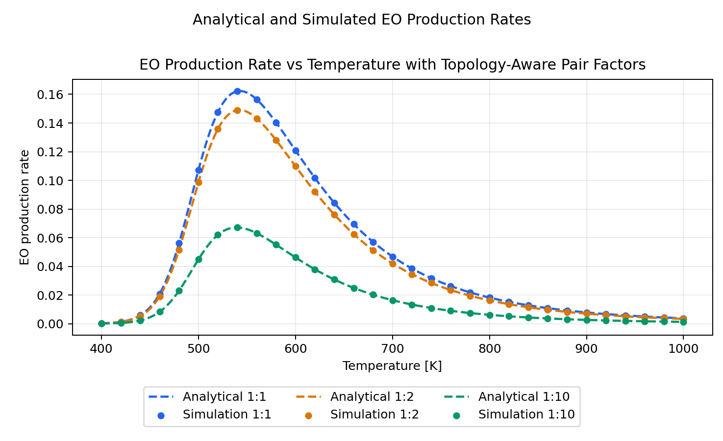
• compares the EO production rate from both

At 500 K, the reproduced EO production rates are:

S1:S2	\(P_{12}\)	Analytical EO rate	Simulated EO rate
1:1	0.500000	0.107178	0.107178
1:2	0.444444	0.0985688	0.0985688
1:10	0.165289	0.0448396	0.0448396

Derived Analyses

The same benchmark input also enables the derived analyses:

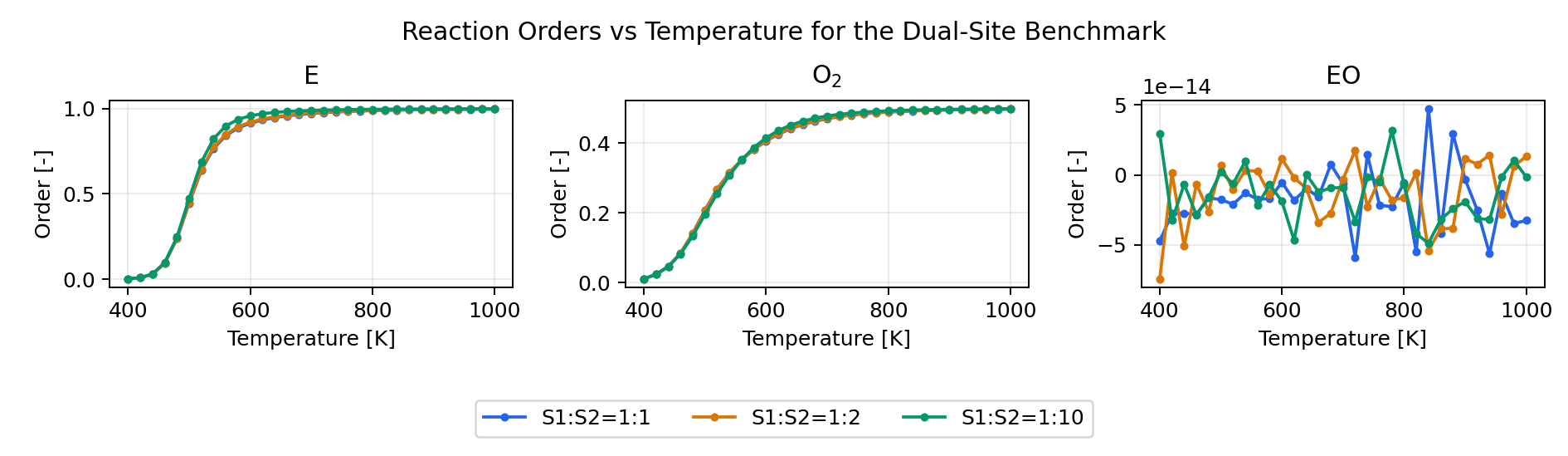
• reaction orders
• apparent activation energy
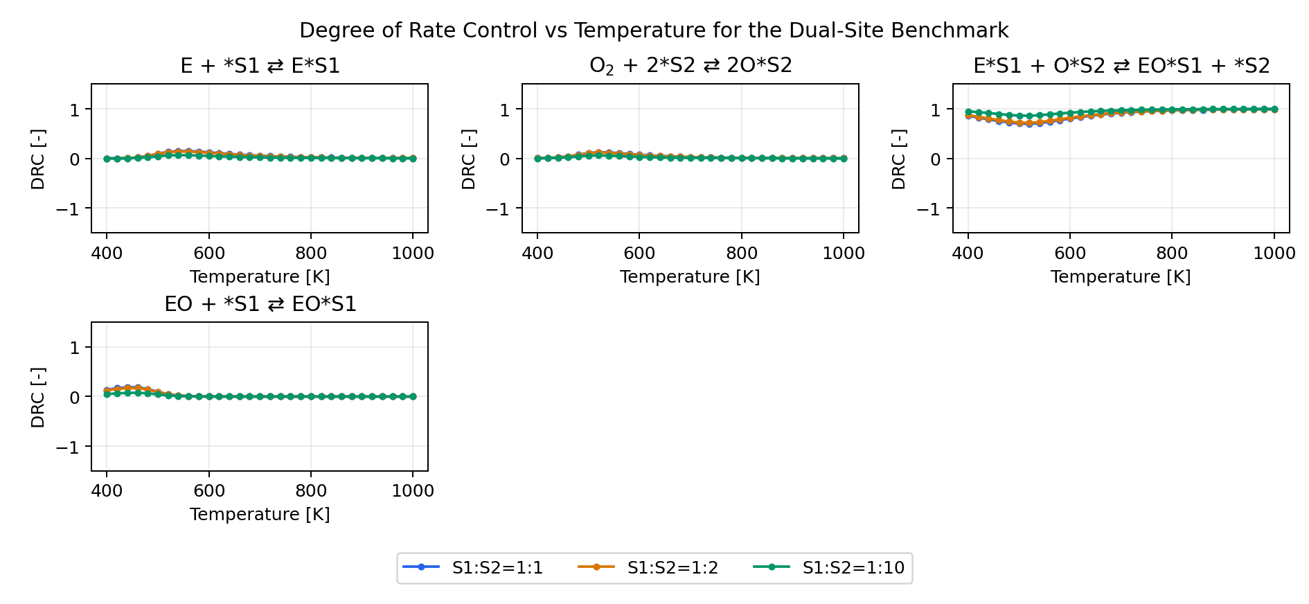
• degree of rate control
• thermodynamic degree of rate control

To make those analyses meaningful, the example tags EO as the key product, marks the surface species for tdrc, and applies drc tags to the elementary steps. The scenario script then produces the analysis outputs for the same 1:1, 1:2, and 1:10 site-ratio cases.

Reaction Orders

Apparent Activation Energy

Degree of Rate Control