Tolerance Analysis

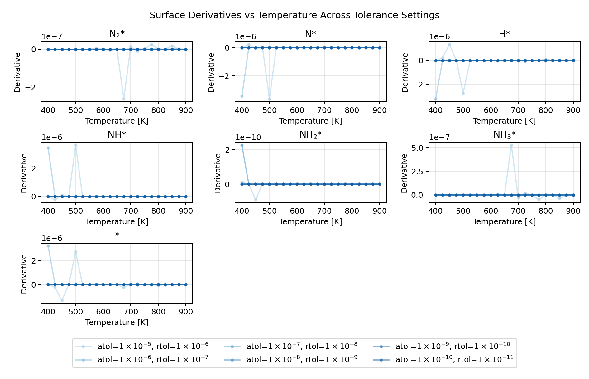
This case study compares six solver-tolerance settings for the ammonia wildcard plotting scenario. For each subsequent run, both atol and rtol were relaxed by one order of magnitude, starting from the strictest reference setting \(a_{\text{tol}} = 1 \times 10^{-10}\) and \(r_{\text{tol}} = 1 \times 10^{-11}\).

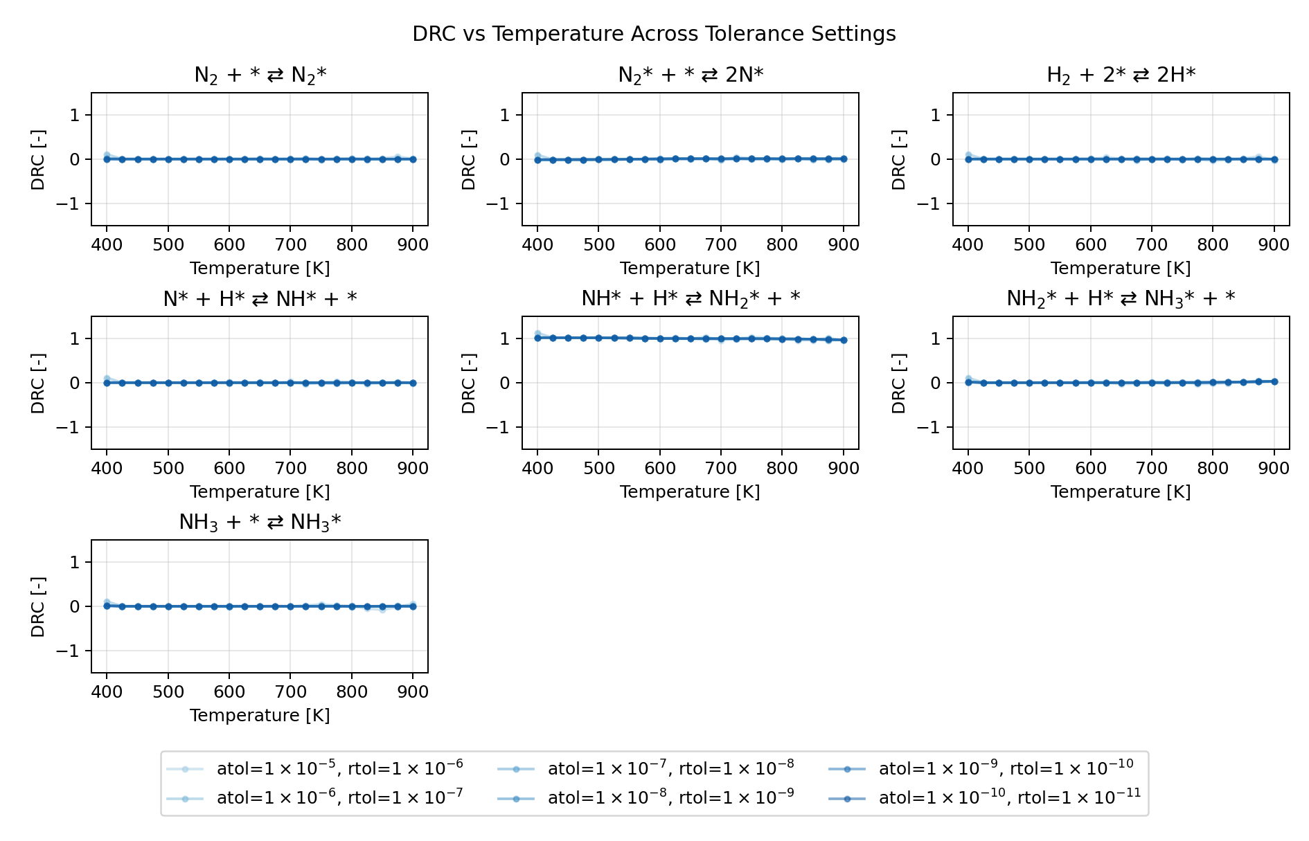
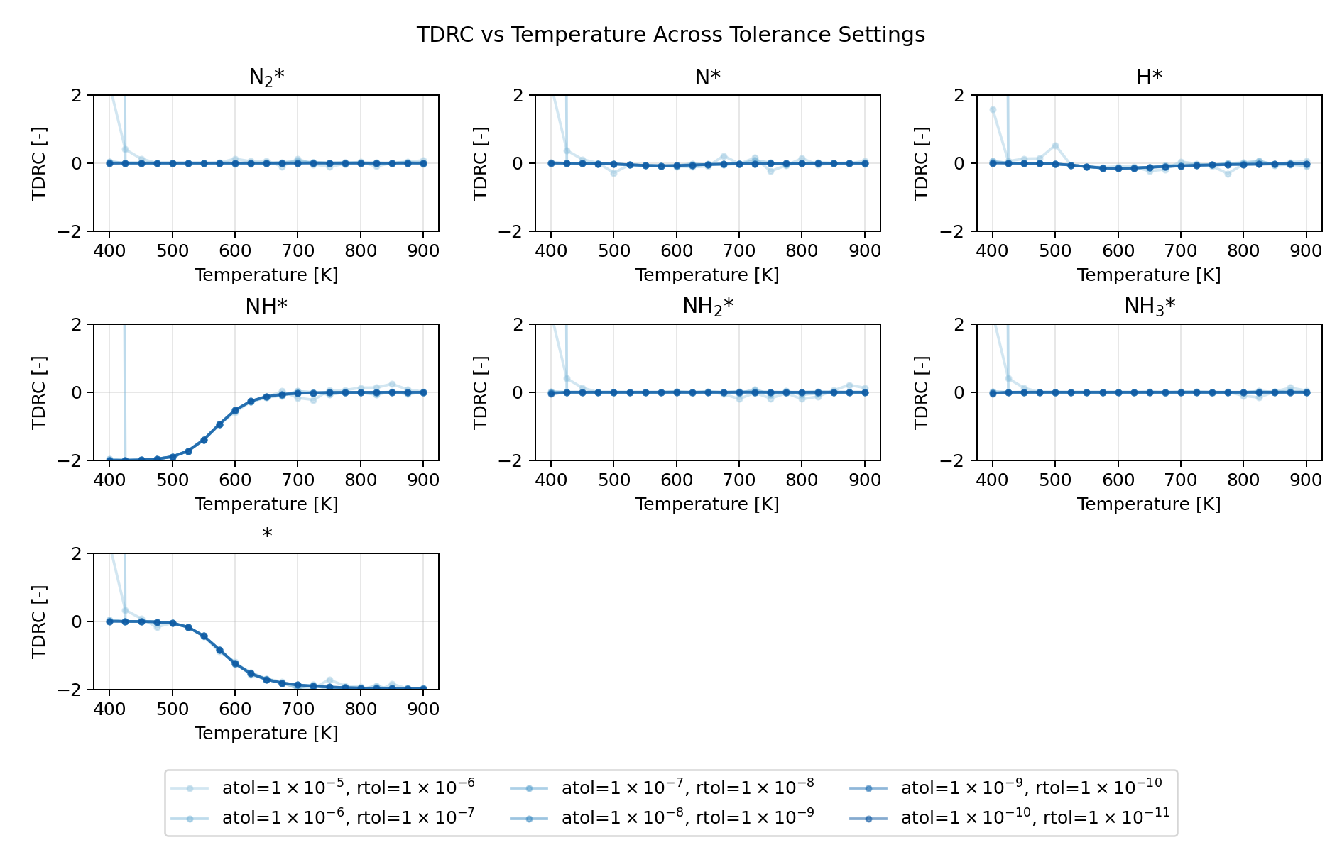
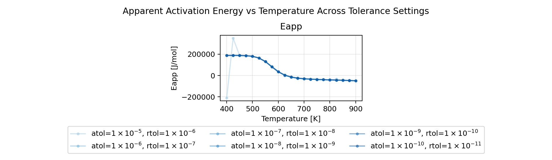
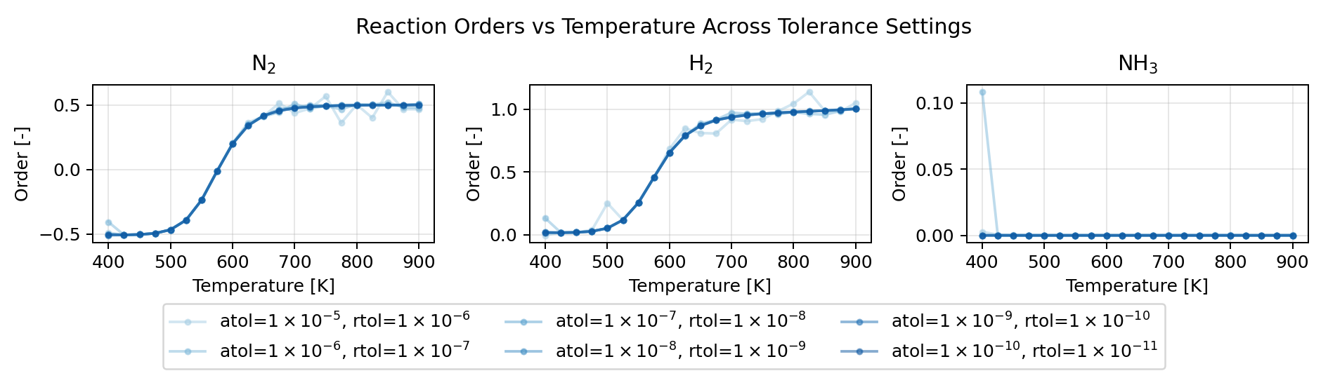
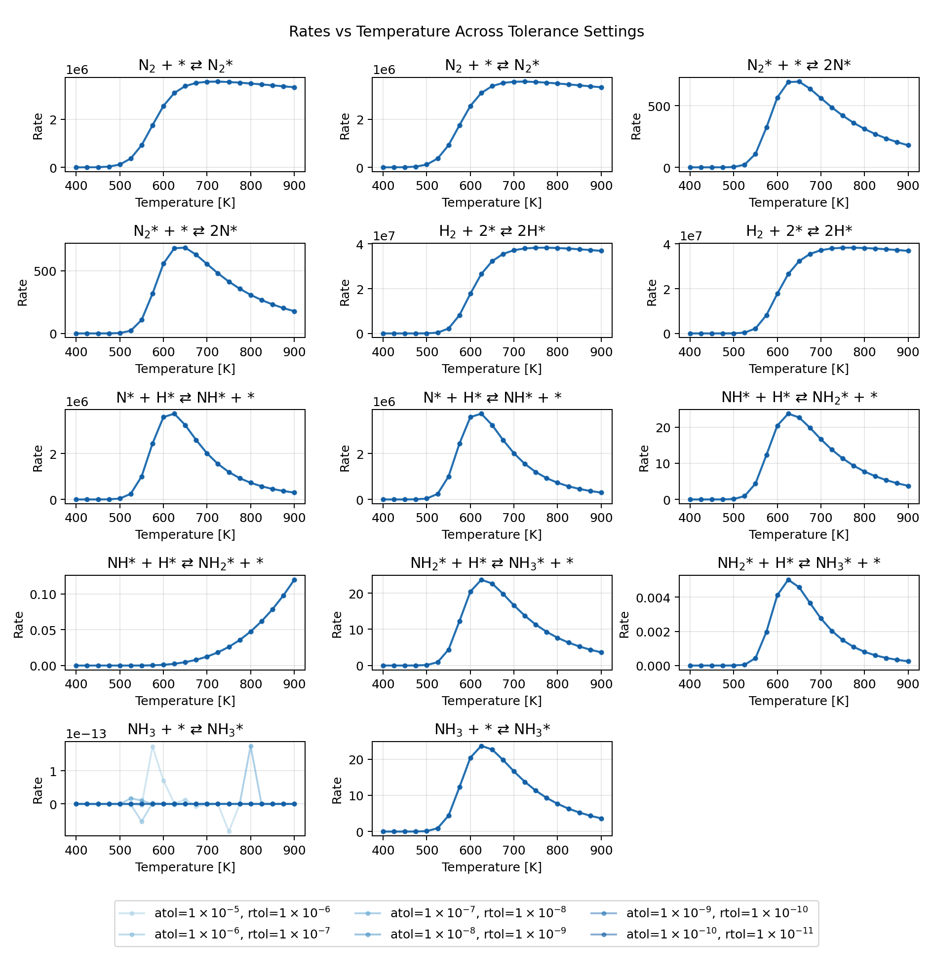
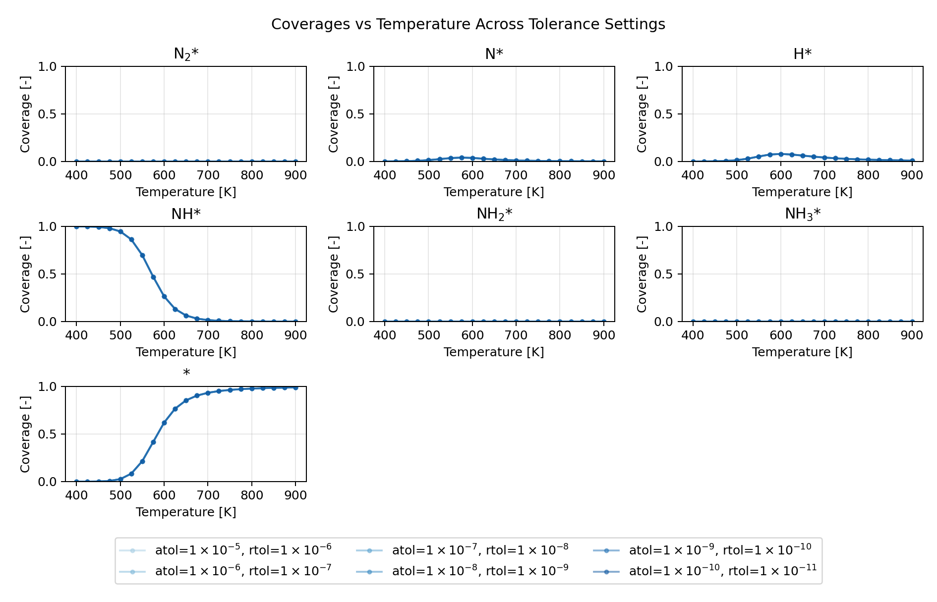
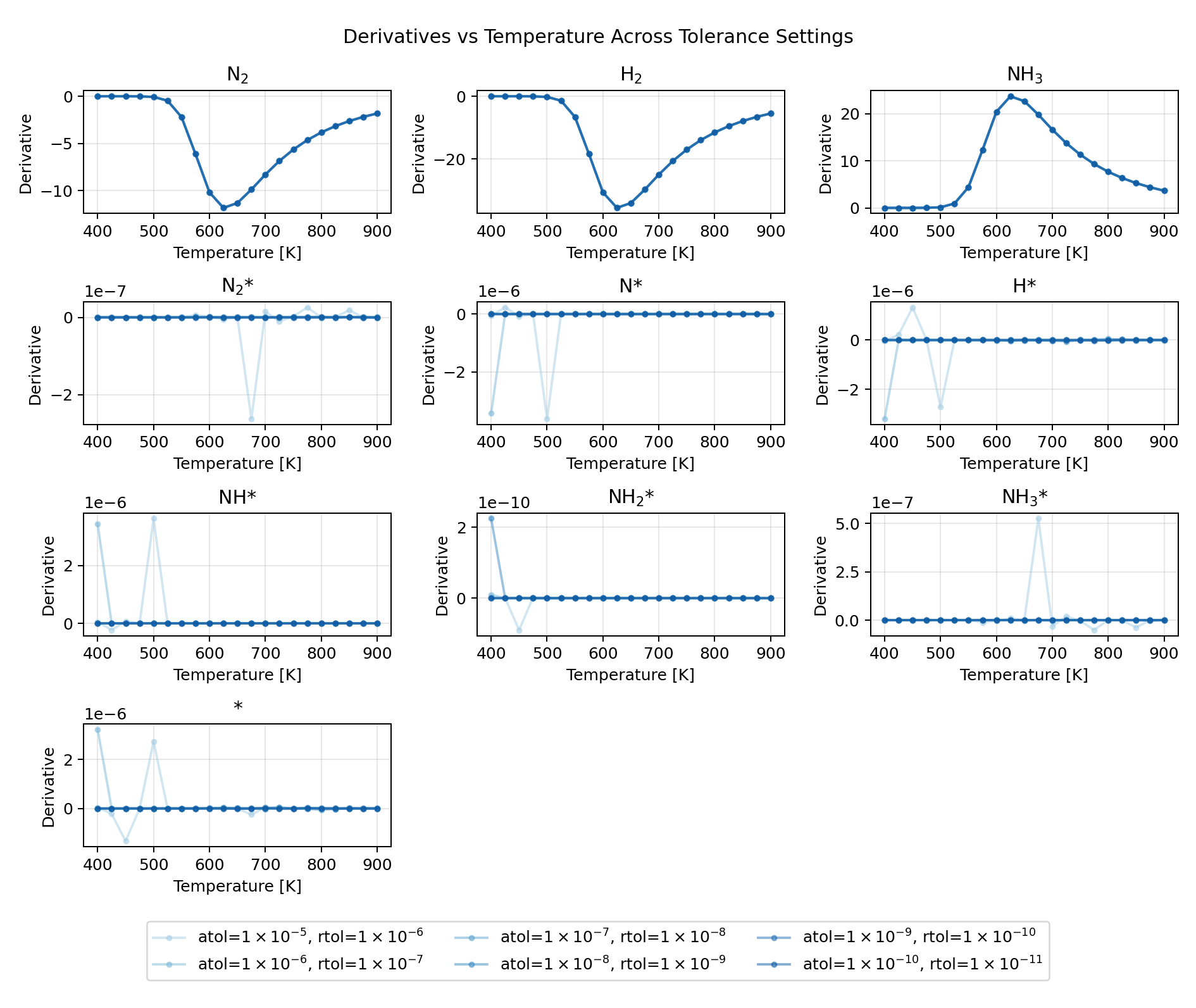
The figures below compare how rates, coverages, derivatives, degree of rate control (DRC), thermodynamic degree of rate control (TDRC), apparent activation energy, and reaction orders evolve as a function of temperature across the full tolerance sweep.

Based on a detailed comparison of the plotted trends and the representative derivative values, the practical sweet spot in this study lies roughly around \(a_{\text{tol}} = 1 \times 10^{-7}\) and \(r_{\text{tol}} = 1 \times 10^{-8}\). At that setting, the results remain close to the stricter reference runs while avoiding the much larger deviations that appear once the tolerances are relaxed further.

Scenario Input

The full reproduction input is also available at tests/scenarios/tolerance/input.mkx.

# Ammonia synthesis solver tolerance analysis.
#
# This scenario-local input reproduces the tolerance sweep case study.

let asite = 1e-20
let hk_n2  = {Asite=asite, m=28, theta=1.0, sigma=2, S=1.0}
let hk_h2  = {Asite=asite, m=2,  theta=85.4, sigma=2, S=1.0}
let hk_nh3 = {Asite=asite, m=17, theta=1.0, sigma=3, S=1.0}

let surf_fast = {Vf=1e13, Vb=1e13}
let surf_slow = {Vf=1e13, Vb=1e13}

components {
  N2   {phase=gas, init=0.20, role=reactant},
  H2   {phase=gas, init=0.60, role=reactant},
  NH3  {phase=gas, init=0.00, role=product, tags=[key]},

  N2*  {phase=surface, init=0.00, tags=[tdrc]},
  N*   {phase=surface, init=0.00, tags=[tdrc]},
  H*   {phase=surface, init=0.00, tags=[tdrc]},
  NH*  {phase=surface, init=0.00, tags=[tdrc]},
  NH2* {phase=surface, init=0.00, tags=[tdrc]},
  NH3* {phase=surface, init=0.00, tags=[tdrc]},
  *    {phase=surface, init=1.00, tags=[tdrc, emptysite]}
}

reactions {
  {N2}+{*}=>{N2*} @ HertzKnudsenDefault(*hk_n2, Edes=70e3) {tags=[drc]},
  {N2*}+{*}=>2{N*} @ ArrheniusDefault(*surf_fast, Eaf=60e3, Eab=85e3) {tags=[drc]},
  {H2}+2{*}=>2{H*} @ HertzKnudsenDefault(*hk_h2, Edes=55e3) {tags=[drc]},
  {N*}+{H*}=>{NH*}+{*} @ ArrheniusDefault(*surf_fast, Eaf=45e3, Eab=65e3) {tags=[drc]},
  {NH*}+{H*}=>{NH2*}+{*} @ ArrheniusDefault(*surf_slow, Eaf=115e3, Eab=95e3) {tags=[drc]},
  {NH2*}+{H*}=>{NH3*}+{*} @ ArrheniusDefault(*surf_fast, Eaf=35e3, Eab=75e3) {tags=[drc]},
  {NH3}+{*}=>{NH3*} @ HertzKnudsenDefault(*hk_nh3, Edes=80e3) {tags=[drc]}
}

simulation {
  ammonia_tolerance @ transient_solve(
    model=thermal,
    solver={
      method=cvode_bdf,
      atol=1e-10,
      rtol=1e-11,
      t_end=1e6,
      steady_state_threshold=1e-9,
      jacobian=analytic,
      max_order=8
    },
    conditions=[
      {T=400}, {T=425}, {T=450}, {T=475}, {T=500},
      {T=525}, {T=550}, {T=575}, {T=600}, {T=625},
      {T=650}, {T=675}, {T=700}, {T=725}, {T=750},
      {T=775}, {T=800}, {T=825}, {T=850}, {T=875},
      {T=900}
    ],
    analyses=[
      {type=orders},
      {type=eapp},
      {type=drc},
      {type=tdrc}
    ]
  )
}

output {
  formats=[tabdelim, hdf5],
  folder="tests/scenarios/tolerance/results/base_placeholder"
}

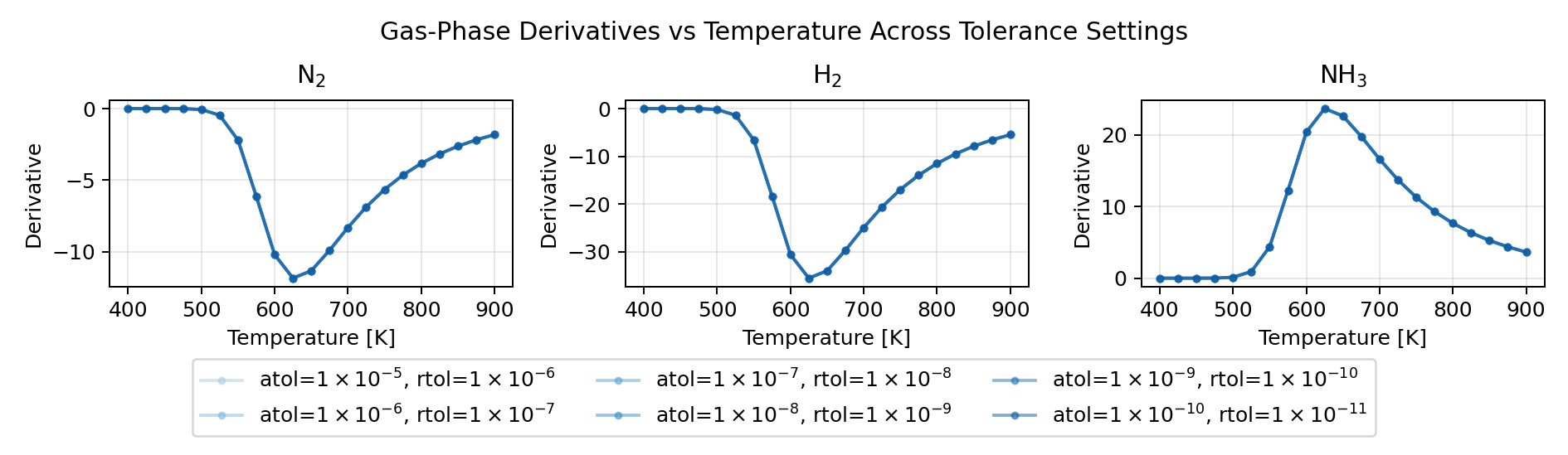
Representative Derivative Table

The strictest run reaches its maximum NH3 formation derivative at 625 K, which we take here as a representative operating point. The table below lists the gas-phase derivatives at that temperature for all six tolerance settings.

Table 1: Gas-phase derivatives at the optimal temperature (625 K) across the six tolerance settings. The optimal temperature is defined here as the temperature of maximum NH3 derivative in the strictest run.

Tolerance setting	`N2`	`H2`	`NH3`
`1e-10 / 1e-11`	`-1.184265e+01`	`-3.552795e+01`	`2.368530e+01`
`1e-9 / 1e-10`	`-1.184266e+01`	`-3.552797e+01`	`2.368532e+01`
`1e-8 / 1e-9`	`-1.184265e+01`	`-3.552795e+01`	`2.368530e+01`
`1e-7 / 1e-8`	`-1.184326e+01`	`-3.552977e+01`	`2.368652e+01`
`1e-6 / 1e-7`	`-1.184249e+01`	`-3.552748e+01`	`2.368499e+01`
`1e-5 / 1e-6`	`-1.183390e+01`	`-3.550171e+01`	`2.366781e+01`

Calculation Times

The runtime drops sharply as the solver tolerances are relaxed, which is what makes the intermediate settings attractive in practice.

Table 2: Approximate wall-clock calculation times across the six tolerance settings, estimated from the first and last timestamps in each run log.